Writing Screener Criteria | Data Saham Indonesia

Versions 1.3.03 – 1.3.05 of the Data Saham Indonesia app added the Stock Screener and Stock Scoring features. This article covers how to write criteria for both.

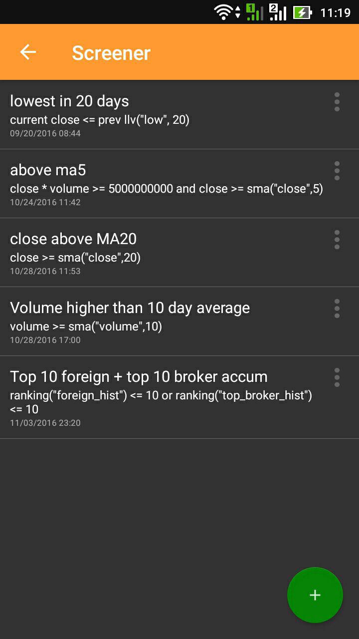
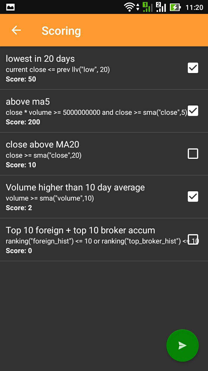
The Stock Screener in the Data Saham Indonesia app Stock Scoring in the Data Saham Indonesia app

Trade US stocks or crypto too? The same formula language, minus the IDX-only broker, foreign-flow and order-book variables, works in our other app, Profit Scanner, for screeners and alerts on US stocks and crypto.

Boolean Expression

Screener criteria are written as a mathematical formula called a Boolean Expression (BE) — a logical statement the system evaluates to one of two values: true or false.

Examples:

4 == 4                   ==> true
4 == 3 + 1               ==> true
4 > 5                    ==> false
true and false           ==> false
true or false            ==> true
4 == 4 and 4 == 3 + 1    ==> true

== is the operator for testing equality of values.

The screener evaluates your Boolean Expression against every stock listed on the Indonesia Stock Exchange, then shows those that return true.

For example:

prev hourly close <= current hourly close

Returns stocks whose close on the previous hourly candle is less than or equal to the close on the current hourly candle.

prev hourly close <= current hourly close AND hourly close >= hourly sma("close", 5)

The same criterion, AND close above the hourly MA5.

Screener criteria are flexible. They can be as simple as:

open < close

or as involved as:

hourly high > prev hourly hhv("high", 100) and
hourly close > hourly open and
index macd_histogram > 0 and
high < bollinger_top

Expression hierarchy

Boolean Expressions and Arithmetic Expressions are both derived from Expression. An Arithmetic Expression is a statement that produces a single value in the set of real numbers. Expression itself is defined as “anything that produces a single value”.

The hierarchy is as follows:

Expression :
  - Boolean Expression (BE)
      - Boolean Value       : true, false
      - Bracket Expression  : ( BE )
      - Boolean Operation   : and, or, not
      - Arithmetic Comparison : >= , <= , > , < , == , !=
      - Boolean Function    : code_index("<index code>")
      - Cross Operation     : E cross_up E, E cross_down E
  - Arithmetic Expression (E)
      - Numeric Expression
      - Arithmetic Operation : * , / , + , -
      - Bracket Expression   : ( E )
      - Stock Expression

In this document and in the criteria composer, E is shorthand for Arithmetic Expression.

Number notation

Numeric values can be written with a unit suffix, so large numbers stay short and readable:

K = thousand   1,000
M = million    1,000,000
B = billion    1,000,000,000
T = trillion   1,000,000,000,000

Examples:

value > 1B          ==> transaction value above 1 billion rupiah
market_cap >= 10T   ==> market capitalisation of at least 10 trillion rupiah
volume > 500K       ==> volume above 500 thousand

Writing the number in full still works — 1B and 1000000000 are the same value.

Conditional operator

The ? : operator picks one of two values based on a condition:

<condition> ? <value if true> : <value if false>

It is most useful inside a subformula, because it turns a condition into a number that can then be summed or averaged.

sum("close > open ? 1 : 0", 20)     ==> how many green candles in 20 bars
sma("volume > 1B ? 1 : 0", 10)      ==> proportion of high-volume days
sum("close > prev close ? volume : 0", 5)  ==> volume on up days only

To simply count how many times a condition holds, the count function is shorter:

count("close > open", 20)           ==> equivalent to the first example above

Stock Expression

The most important part of a screener criterion is the Stock Expression, which is derived from Arithmetic Expression.

Its structure is:

E: stock_expression: [candle_selector] [timeframe] [target] <stock_attr>
E: stock_expression: [candle_selector] [timeframe] [target] <stock_function>
E: stock_expression: <stock_fundamental_attr>
E: stock_expression: <bid_offer_variables>

candle_selector

candle_selector: prev_N, ..., prev_3, prev_2, prev, current
default: current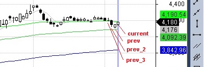

Candle selector illustration

prev_N can also be written without the underscore: prev2 close is the same as prev_2 close.

A whole formula on an earlier bar: `prev()`

prev placed before a name moves that one value back a bar. To move a whole formula back, put it in brackets after prev:

prev(close - open)             ==> the body of the previous candle
prev(sma(20) * 1.02)           ==> the same as prev sma(20) * 1.02
prev(close > open)             ==> true when the previous candle was green
prev_3(close)                  ==> the close three bars back, the same as prev_3 close
prev3(high - low)              ==> the range of the candle three bars back
prev(prev(close))              ==> the same as prev_2 close

Every value inside the brackets moves back together, each on its own timeframe: prev(weekly close > weekly open) asks whether last week’s candle was green.

prev() takes a single formula. For more than one bar back, put the number in the name: prev_3(close), not prev(close, 3). The same thing can also be written as val(formula, N):

val(close - open, 1)           ==> the same as prev(close - open)
val(close, 5)                  ==> the same as prev_5(close)

A plain number has no earlier bar, so prev(20) is an error. To compare against an indicator’s previous value, write prev sma(20).

timeframe

timeframe: yearly, quarterly, monthly, weekly, daily,
           4hour, 3hour, 2hour, hourly,
           45min, 30min, 15min, 10min, 5min, 3min, 2min, 1min
default: daily

30min close > 30min sma(20)    ==> above the MA 20 of the 30-minute chart
2hour rsi(14) < 30             ==> oversold on the 2-hour chart

target

target: stock, sector, index
default: stock

stock — the chart of the stock itself. For TLKM and BMRI, target stock selects the TLKM and BMRI charts.
sector — the chart of the sectoral index. For TLKM and BMRI, target sector selects the INFRA and FINANCE index charts.
index — the composite index chart for that stock. For TLKM and BMRI, target index selects COMPOSITE (^JKSE).

Writing parameters

Parameters with a default value may be omitted. In a Stock Expression, only stock_attr is required.

current daily stock close == close                ==> true
current daily stock close == daily close          ==> true
current daily stock close == stock close          ==> true
current daily stock close == current daily close  ==> true

But when parameters are written, they must follow the order defined above:

stock daily close    ==> error
daily current close  ==> error
current daily close  ==> OK

stock_attr list

open, high, low, close, volume
macd, macd_signal, macd_histogram
ppo, ppo_signal, ppo_histogram, pvo
ao, chaikin_osc, tsi, mass_index, trix
aroon_up, aroon_down, aroon_osc
donchian_up, donchian_down, donchian_mid
rsi, stoch_k, stoch_d, stochrsi, atr, adx, pdx, ndx, cci, uo, roc, william_r, mfi, cmf
up_fractal, down_fractal
alligator_jaw, alligator_teeth, alligator_lips, alligator_ao, alligator_ac
bollinger_top, bollinger_bottom, bollinger_mean, bollinger_bandwidth,
bollinger_percent_b, bollinger_percent_b_avg
value, top_broker, foreign, top_broker_hist, foreign_hist
dto_stochk, dto_stochd, obv, adl, sar
pivot_s1, pivot_s2, pivot_s3, pivot_r1, pivot_r2, pivot_r3
camarilla_h1, camarilla_h2, camarilla_h3, camarilla_h4
camarilla_l1, camarilla_l2, camarilla_l3, camarilla_l4
mid_price, hlc3, ohlc4, avg_price, tick, freq, change_percent
up_fractal_index, down_fractal_index
frequency_analyzer, mfv, ma_net_buy_sell_signal_count
projected_volume, projected_value
iep, iev, time_progress
open_date, open_time, close_date, close_time

Short forms with a standard period

The indicator names above can be written without brackets. The short form uses that indicator’s standard period, so ppo is the same as ppo(12, 26) and ao the same as ao(5, 34).

Short form	Standard period
`rsi`, `atr`, `adx`, `pdx`, `ndx`, `cci`, `mfi`, `william_r`	14
`roc`	12
`cmf`	21
`trix`	15
`stochrsi`	14
`dto_stochk`, `dto_stochd`	14, 8, 5, 3
`stoch_k`, `stoch_d`	15, 3, 3
`uo`	7, 14, 28
`macd`, `ppo`, `pvo`	12, 26
`macd_signal`, `macd_histogram`, `ppo_signal`, `ppo_histogram`	12, 26, 9
`ao`	5, 34
`chaikin_osc`	3, 10
`tsi`	25, 13
`mass_index`	9, 25
`aroon_up`, `aroon_down`, `aroon_osc`	25
`donchian_up`, `donchian_down`, `donchian_mid`	20
`bollinger_*`	20, 2
`sar`	0.02, 0.2
`supertrend`, `supertrend_dir`	10, 3
`chandelier_long`, `chandelier_short`, `chandelier_dir`	22, 3

When you need a different period, write the full function form:

rsi < 30                ==> uses the standard period, rsi(14)
rsi(7) < 30             ==> a period of your own choosing

Moving averages also have a numbered form — the function name followed by the period:

sma20                   ==> the same as sma("close", 20)
ema50, wma10, aema20, dema20, tema50, vwma20

Shorthand names

The names typed most often also have a shorthand, and a few accept the name used on TradingView or AmiBroker:

Shorthand	Full name
`xu`, `crossover`	`cross_up`
`xd`, `crossunder`	`cross_down`
`dtok`, `dtod`	`dto_stochk`, `dto_stochd`
`stok`, `stod`	`stoch_k`, `stoch_d`
`pdi`, `mdi`	`pdx`, `ndx`
`macdh`	`macd_histogram`
`bbtop`, `bbbot`	`bollinger_top`, `bollinger_bottom`
`willr`, `wpr`	`william_r`
`nbsa`	`foreign_hist` (net foreign buy/sell)
`vol`	`volume`
`hl2`	`mid_price`

A shorthand works anywhere its full name does, with parameters, a timeframe or prev:

stok(14, 3) xu stod(14, 3, 3)
weekly dtok(14, 14, 3, 3) > weekly dtod(14, 14, 3, 3)
vol > 2 * sma("volume", 20)
close > bbtop and prev nbsa > 0

Underscores are optional. Every name that contains an underscore can also be written without it, which saves a keystroke on a phone keyboard:

changepercent > 2          ==> the same as change_percent > 2
codeindex("LQ45")          ==> the same as code_index("LQ45")
macdhistogram > 0          ==> the same as macd_histogram > 0
top5bidvolume > top5offervolume

stock_attr definitions

open, high, low, close, volume — the open, high, low, close and volume of the candlestick chart
macd, macd_signal, macd_histogram — values from the MACD(12,26,9) chart; macd_histogram = macd − macd_signal
rsi — value from the RSI(14) chart
stoch_k, stoch_d — values from the Stochastic(15,3,3) chart
stochrsi — value from the StochRSI(9,6) chart
atr — value from the ATR(14) chart
adx, pdx, ndx — values from the ADX(14) chart; pdx is the DI+ line and ndx the DI− line
cci — value from the CCI(14) chart
uo — value from the UO(7,14,28) chart
roc — value from the ROC(12) chart
william_r — value from the WilliamsR(14) chart
mfi — value from the MFI(14) chart
cmf — value from the CMF(21) chart
alligator_jaw, alligator_teeth, alligator_lips, alligator_ao, alligator_ac — values from the Alligator(13,8,5) chart
bollinger_top, bollinger_bottom, bollinger_mean, bollinger_bandwidth, bollinger_percent_b, bollinger_percent_b_avg — values from the Bollinger(20,2) chart
value — total transaction value of the stock
top_broker — cumulative top broker transactions (current top_broker = prev top_broker + current top_broker_hist)
foreign — cumulative foreign transactions (current foreign = prev foreign + current foreign_hist)
top_broker_hist — value from the top broker transaction histogram, in shares
foreign_hist — value from the foreign transaction histogram, in shares
adl — Accumulation/Distribution Line, a running total of money flow volume: the position of the close within the daily range, multiplied by volume. It rises when closes sit near the high and falls when they sit near the low
dto_stochk, dto_stochd — values from the DTOStoch(8,5,3) chart
sar — value from the SAR(0.02,0.2) chart
mid_price — mid_price = (high + low) / 2; also written hl2
hlc3 — (high + low + close) / 3, the typical price; the same value as vwap
ohlc4 — (open + high + low + close) / 4
tick — the exchange price fraction (price < 200 : 1 ; 200–500 : 2 ; 500–2000 : 5 ; 2000–5000 : 10 ; > 5000 : 25)
vwap — vwap = (high + low + close) / 3
avg_price — the average transaction price on that bar; avg_price = value / volume
freq — the number of transactions on that bar
change_percent — price change against the previous close, as a percentage
camarilla_h1 … camarilla_h4, camarilla_l1 … camarilla_l4 — Camarilla pivot levels
up_fractal_index, down_fractal_index — bars elapsed since the last upper or lower fractal formed
frequency_analyzer — volume / freq³, a measure of average transaction size. High values indicate trading dominated by large orders
mfv — money flow volume, the position of the close within the daily range multiplied by volume
ma_net_buy_sell_signal_count — buy signals minus sell signals across 12 moving averages (SMA and EMA at periods 5, 10, 20, 50, 100, 200). Ranges from −12 to +12
projected_volume, projected_value — estimated volume and transaction value through to the session close, based on the pace of trading so far
iep, iev — indicative equilibrium price and volume during the pre-opening session
time_progress — the proportion of the trading session elapsed, 0 to 1
open_date, close_date, open_time, close_time — the opening and closing date and time of the bar

A note on adl, top_broker and foreign. All three are cumulative, counted from the oldest bar available, so their values are relative: they cannot be compared between stocks, nor stored and compared again on a different day. What carries meaning is the direction — against the previous bar, or against an average of the value itself.

adl > prev adl                       ==> accumulation increased today
adl > sma("adl", 20)                 ==> accumulation above its own average
prev adl < prev sma("adl", 20) and adl > sma("adl", 20)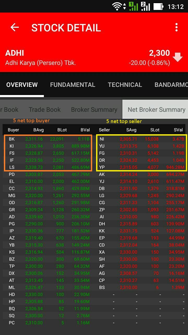

top_broker_hist = 5 top net buyers minus 5 top net sellers

top_broker_hist = [5 top net buyer] - [5 top net seller]

stock_function list

A stock_function is a function of a stock_attr.

sma(n), sma(subformula,n)
ema(n), ema(subformula,n)
aema(n), aema(subformula,n)
med(n), med(subformula,n)
highest(subformula,n), hhv(subformula,n)
lowest(subformula,n), llv(subformula,n)
ranking(subformula,n)
ranking_per_sector(subformula,n)
roc(n)
macd(fast_period,slow_period)
macd_signal(fast_period,slow_period,signal_period)
macd_histogram(fast_period,slow_period,signal_period)
sum(subformula,n)
supertrend(atr_period,multiplier), supertrend_dir(atr_period,multiplier)
chandelier_long(period,multiplier), chandelier_short(period,multiplier), chandelier_dir(period,multiplier)
cum(subformula)
since(date)
vwap(n)
vwma(n)
wma(n), wma(subformula,n)
linreg(n), linreg(subformula,n)
slope(n), slope(subformula,n)
linreg_r2(n), linreg_r2(subformula,n)
cci(n)
atr(n)
adx(n)
pdx(n)
ndx(n)
stoch_k(lookback_period,k_period)
stoch_d(lookback_period,k_period,d_period)
bollinger_top(period, multiplier)
bollinger_bottom(period, multiplier)
bollinger_mean(period, multiplier)
bollinger_bandwidth(period, multiplier)
bollinger_percent_b(period, multiplier)
bollinger_percent_b_avg(period, multiplier)
stdev_p(n), stdev_p(subformula,n)
stdev_s(n), stdev_s(subformula,n)
stdev(n), stdev(subformula,n)
rsi(n)
stochrsi(period,dtostoch_period,dtostoch_k_period,dtostoch_d_period)
dto_stochk(period,dtostoch_period,dtostoch_k_period,dtostoch_d_period)
dto_stochd(period,dtostoch_period,dtostoch_k_period,dtostoch_d_period)
mfi(n)
cmf(n)
chaikin_osc(fast_period, slow_period)
aroon_up(period)
aroon_down(period)
aroon_osc(period)
dema(period)
tema(period)
trix(period)
mass_index(ema_period, sum_period)
tsi(long_period, short_period)
donchian_up(period)
donchian_down(period)
donchian_mid(period)
ppo(fast_period, slow_period)
ppo_signal(fast_period, slow_period, signal_period)
ppo_histogram(fast_period, slow_period, signal_period)
pvo(fast_period, slow_period)
ao(fast_period, slow_period)

abs(x)
pow(x, y)
sqrt(x)
exp(x)
ln(x)
log10(x), log(x, base)
ceil(x), ceil(x, decimals)
floor(x), floor(x, decimals)
round(x), round(x, decimals)
trunc(x, decimals)
min(a, b, ...), max(a, b, ...), avg(a, b, ...)

count(subformula, n)
hhvbars(subformula, n)
llvbars(subformula, n)

pivot_high(k), pivot_high(k, n)
pivot_low(k), pivot_low(k, n)
pivot_high_bars(k), pivot_high_bars(k, n)
pivot_low_bars(k), pivot_low_bars(k, n)

trade_book(price)
freq(price)
tick_up(price), tick_down(price)

stock_function definitions

sma("<stock_attr>", N) — simple moving average of a stock_attr over N bars.

sma("close", 5)            ==> daily MA5 of close
hourly sma("volume", 20)   ==> hourly MA20 of volume

ema("<stock_attr>", N) — exponential moving average of a stock_attr over N bars.

ema("close", 5)            ==> daily EMA5 of close
hourly ema("volume", 20)   ==> hourly EMA20 of volume

aema("<stock_attr>", N) — an exponential moving average that stays more accurate on limited history. Written exactly like ema.

aema("close", 5)           ==> daily EMA5 of close
aema("volume * close", 20) ==> EMA20 of transaction value

Use aema when your criterion uses a long period or works on sharply fluctuating values — volume, price differences, ratios. For short periods on price, the two give practically identical results.

If you already have screeners or alerts running on ema, there is no need to change them. ema remains available and its behaviour is unchanged.

highest("<stock_attr>", N) / hhv("<stock_attr>", N) — the highest value of a stock_attr over N bars.

daily hhv("high", 5)    ==> 5 day highest high daily
hourly hhv("close", 5)  ==> 5 hour highest close hourly

lowest("<stock_attr>", N) / llv("<stock_attr>", N) — the lowest value of a stock_attr over N bars.

daily llv("low", 5)     ==> 5 day lowest low daily
hourly llv("close", 5)  ==> 5 hour lowest close hourly

ranking("<stock_attr>", N) — the rank of a stock_attr across all stocks, where rank 1 is the highest value. To order from lowest to highest instead, multiply the stock_attr by −1.

ranking("value") <= 10       ==> the top 10 stocks by transaction value
ranking("roc") <= 10         ==> the 10 stocks with the highest ROC
ranking("roc * -1") <= 10    ==> the 10 stocks with the lowest ROC

roc(period) — value from the Rate of Change (ROC) chart.

roc(12)  ==> value of roc(12)

macd(fast_period, slow_period), macd_signal(...), macd_histogram(...) — values from the macd, macd_signal and macd_histogram charts.

macd(12, 26)                 ==> value of macd(12, 26)
macd_signal(12, 26, 9)       ==> value of macd signal(12, 26, 9)
macd_histogram(12, 26, 9)    ==> value of macd histogram(12, 26, 9)

sum("<stock_attr>", N) — the sum of a stock_attr over N bars.

sum("foreign", 5)  ==> total foreign accumulation over the last 5 days

cum("<expression>") — the sum of an expression across every bar available, the equivalent of Cum() in AmiBroker or MetaStock.

cum("volume")                     ==> accumulated volume across all data
cum("close > open ? 1 : 0")       ==> the number of green candles across all data

Because each calculation reads only a bounded stretch of recent bars, the total starts from the oldest bar available rather than from the day the stock was first listed. Its value is therefore relative: it cannot be compared between stocks, nor stored and compared again on a different day — the same caveat that applies to adl, top_broker and foreign.

For most purposes sum with an explicit period is the more useful of the two, since its result is comparable between stocks:

sum("volume", 20)                 ==> total volume over the last 20 bars

since("<date>") — the number of bars from that date up to the current bar. It is rarely used on its own; its purpose is to stand in for the period argument of another function, so that a calculation is bounded by a date rather than by a bar count.

The date can be written in several forms:

since("2026/01/01")     ==> YYYY/MM/DD
since("01/01/2026")     ==> DD/MM/YYYY
since("20260101")       ==> YYYYMMDD

A hyphenated form such as 2026-01-01 is not recognised.

Examples:

sum("volume", since("2026/01/01"))          ==> accumulated volume year to date
hhv("high", since("2026/01/01"))            ==> the highest price year to date
llv("low", since("2026/07/01"))             ==> the lowest price since the start of July
count("close > open", since("2026/01/01"))  ==> green candles year to date

If the date requested is older than all the data held, the result is the number of bars available — the calculation stops at the oldest bar rather than at the date you wrote.

Because since can return a large number, pair it with functions that have no tight period limit: sum, sma, hhv, llv, count and stdev. On functions such as ema or trix, a long date range can exceed the accurate period limit and return an empty value. See the accurate period limits table.

vwap(N) — value from the Volume-Weighted Average Price indicator.

vwap(N) = sum("volume * (high + low + close) / 3", N) / sum("volume", N)

vwap(5)  ==> vwap over the last 5 days

vwma(N) — Volume Weighted Moving Average, a close-price average weighted by volume. Unlike vwap, the weighting is applied to the close.

vwma(20)                ==> 20-period VWMA
close > vwma(20)        ==> price above VWMA20

wma(N) and wma(subformula, N) — Weighted Moving Average, an average with rising weights: the newest bar carries weight N, the oldest weight 1. It responds to a change in price faster than sma over the same period.

wma(20)                 ==> 20-period WMA
wma("volume", 20)       ==> 20-period WMA of volume
close > wma(20)

linreg(N) and linreg(subformula, N) — the value of the linear regression line through the last N bars, read at the current bar. That line is the straight line closest to every point in the range, not merely a line joining the first and last.

linreg(20)              ==> the 20-bar regression line at the latest bar
close > linreg(20)      ==> price sits above its own regression line

slope(N) and slope(subformula, N) — the gradient of that same line, in price units per bar. Positive when the line rises, negative when it falls.

slope(20) > 0                        ==> the 20-bar trend is rising
slope(20) > slope(50)                ==> the shorter trend is steeper
prev slope(20) < 0 and slope(20) > 0 ==> the gradient has just turned up

Because it is measured in price per bar, slope cannot be compared directly between stocks trading at very different prices. For screening across the market, convert it to a percentage first:

slope(20) / close * 100 > 0.5        ==> rising by more than 0.5% per bar

slope needs at least 2 bars; with a period of 1 the result is empty.

linreg_r2(N) and linreg_r2(subformula, N) — how closely price hugs that regression line, between 0 and 1. A value of 1 means every point sits exactly on the line; a value near 0 means the line explains essentially nothing about the movement.

slope gives the direction and steepness of a trend; linreg_r2 gives how much that trend is worth trusting. The two are complementary: two stocks can share almost the same gradient, one climbing tidily, the other wandering and merely finishing higher.

linreg_r2(20) > 0.7                   ==> the last 20 bars follow the line closely
slope(20) > 0 and linreg_r2(20) > 0.7 ==> an orderly uptrend
slope(20) < 0 and linreg_r2(20) > 0.8 ==> a consistent downtrend

Over a completely flat range the result is 0. Like slope, it needs at least 2 bars.

supertrend(atr_period, multiplier), supertrend_dir(atr_period, multiplier) — TradingView’s Supertrend. The line sits below the price while the trend is up and above it while the trend is down; supertrend_dir is 1 in an uptrend and -1 in a downtrend. The parameters are in the order of TradingView’s indicator settings, ATR length then factor: supertrend(10, 3) is “Supertrend 10 3”. (Pine’s ta.supertrend(factor, atrPeriod) takes them the other way round, and its direction is -1 for up.)

supertrend(10, 3)                   ==> the Supertrend line
supertrend_dir(10, 3) == 1          ==> in an uptrend
supertrend_dir(10, 3) cross_up 0    ==> turned up on this bar (buy)
supertrend_dir(10, 3) cross_down 0  ==> turned down on this bar (sell)

chandelier_long(period, multiplier), chandelier_short(period, multiplier), chandelier_dir(period, multiplier) — the Chandelier Exit, as the widely used TradingView script. The long stop hangs multiplier ATR below the highest close of period bars and only moves up; the short stop sits as far above the lowest close and only moves down. chandelier_dir is 1 after a close above the short stop and -1 after a close below the long stop. A third argument of 0 uses the highest high and lowest low instead of closes.

chandelier_long(22, 3)                ==> the stop for a position you hold
close < chandelier_long(22, 3)        ==> the stop was hit
chandelier_dir(22, 3) cross_up 0      ==> turned up on this bar (buy)
chandelier_long(22, 3, 0)             ==> from the highest high instead of the highest close

atr(period), adx(period), cci(period)

atr(14)  ==> value of the atr(14) line
adx(14)  ==> value of the adx(14) line
pdx(14)  ==> value of the DI+ line in adx(14)
ndx(14)  ==> value of the DI- line in adx(14)
cci(20)  ==> value of cci(20)

stoch_k(lookback_period, k_period) / stoch_d(lookback_period, k_period, d_period) — values from the Stochastic Oscillator chart.

stoch_k(15, 3)     ==> Stochastic %K(15, 3)
stoch_d(15, 3, 3)  ==> Stochastic %D(15, 3, 3)

bollinger_*(period, multiplier) — values from the Bollinger Bands chart.

bollinger_top(20, 2)     ==> Bollinger Band top line(20, 2)
bollinger_bottom(20, 2)  ==> Bollinger Band bottom line(20, 2)

stdev_p(n), stdev_s(n) and stdev(n) — the standard deviation over the last N bars: a measure of how widely values are spread around their average. The larger the number, the more volatile the movement.

Two forms are available, following Excel’s own naming:

stdev_p(20)   ==> population standard deviation  (same as Excel's STDEV.P)
stdev_s(20)   ==> sample standard deviation      (same as Excel's STDEV or STDEV.S)
stdev(20)     ==> the same as stdev_s(20)

stdev_p is the form Bollinger Bands use, so it holds that:

stdev_p(20) == bollinger_top(20, 1) - bollinger_mean(20, 1)

The difference between the two is small — around 2.6% at period 20 and 0.5% at period 100 — but it widens at short periods, to roughly 12% at period 5. If you are matching results against a spreadsheet, use stdev. If you are recreating Bollinger bands, use stdev_p.

Without a subformula all three read the closing price. With one, they can be applied to any value:

stdev("volume", 20)         ==> spread of 20-day volume
stdev("high - low", 20)     ==> spread of the daily range
stdev("(close - prev close) / prev close * 100", 20)
                            ==> volatility of daily returns, in percent

Examples:

close > sma("close", 20) + 2 * stdev_p(20)
                            ==> breaking above two standard deviations
stdev("high - low", 20) < stdev("high - low", 60) * 0.7
                            ==> daily range narrowing against the last three months
stdev(20) / sma("close", 20) * 100 < 2
                            ==> volatility below 2% of price

stdev_s and stdev need at least 2 bars; with a period of 1 the result is empty.

rsi(n) — value from the Relative Strength Index chart.

rsi(14)  ==> value of the rsi(14) line

stochrsi(...), dto_stochk(...), dto_stochd(...) — values from the StochRSI chart.

stochrsi(14, 8, 5, 3)    ==> value of the stochrsi(14, 8, 5, 3) line
dto_stochk(14, 8, 5, 3)  ==> the %K line of stochrsi(14, 8, 5, 3)
dto_stochd(14, 8, 5, 3)  ==> the %D line of stochrsi(14, 8, 5, 3)

chaikin_osc(fast_period, slow_period) — the Chaikin Oscillator: the difference between two EMAs of the Accumulation/Distribution Line. It measures accumulation and distribution pressure by taking the position of the close within the daily range, multiplied by volume.

Positive values indicate accumulation pressure, negative values distribution. Zero-line crossings are commonly used as a signal.

chaikin_osc(3, 10)   ==> Chaikin Oscillator with standard periods
chaikin_osc(5, 20)   ==> a slower variant

Example: switching from distribution to accumulation.

prev chaikin_osc(3, 10) < 0 and chaikin_osc(3, 10) > 0

aroon_up(period) and aroon_down(period) — measure how recently the highest or lowest price was reached within the last N periods, not how high the price is.

Values range from 0 to 100:

100 means the high (or low) occurred on the current bar.
0 means it occurred on the oldest bar in the window.

aroon_up(25)     ==> 100 if today is the highest price of the last 25 days
aroon_down(25)   ==> 100 if today is the lowest price of the last 25 days

aroon_osc(period) — the difference between the two, aroon_up minus aroon_down. It ranges from −100 to +100; positive values indicate an upward bias.

aroon_osc(25)    ==> equivalent to aroon_up(25) - aroon_down(25)

The usual periods are 25 (Chande’s default) and 14.

dema(period) and tema(period) — Double and Triple Exponential Moving Average of the close. Both track price faster than a plain EMA of the same period, making them more responsive to changes in direction.

dema(20)                       ==> 20-period DEMA
close > tema(50)               ==> price above TEMA50
prev close <= prev dema(20) and close > dema(20)

trix(period) — the percentage rate of change of a triple-smoothed price. It oscillates around zero: positive indicates upward momentum, negative downward.

trix(15)                       ==> 15-period TRIX
prev trix(15) < 0 and trix(15) > 0    ==> momentum turning up

mass_index(ema_period, sum_period) — detects expansion in the price range (the high-to-low distance), which often precedes a reversal. Standard parameters are mass_index(9, 25).

The common pattern is the reversal bulge: the value rises above 27, then falls back below 26.5.

mass_index(9, 25) > 27
prev mass_index(9, 25) > 27 and mass_index(9, 25) < 26.5

tsi(long_period, short_period) — True Strength Index, measuring the strength and direction of momentum on a scale of −100 to +100. Standard parameters are tsi(25, 13).

tsi(25, 13) > 0                ==> net positive momentum
prev tsi(25, 13) < 0 and tsi(25, 13) > 0

donchian_up(period), donchian_down(period) and donchian_mid(period) — the upper band, lower band and midline of the Donchian Channel: the highest and lowest values over the last N bars.

donchian_up(20)     ==> highest high of the last 20 bars
donchian_down(20)   ==> lowest low of the last 20 bars
donchian_mid(20)    ==> the midpoint of the two

The current bar is included, as with hhv and llv. This means close > donchian_up(20) can never be true — to find a breakout, compare against the previous bar using prev.

close > prev donchian_up(20)     ==> upside breakout
close < prev donchian_down(20)   ==> downside breakdown

ppo(fast_period, slow_period) — Percentage Price Oscillator, MACD expressed as a percentage. Because the unit is a percentage, values are comparable across stocks trading at very different price levels.

ppo(12, 26)                         ==> PPO with standard periods
ppo(12, 26) > 0                     ==> short-term trend above long-term
prev ppo(12, 26) < 0 and ppo(12, 26) > 0

ppo_signal(fast_period, slow_period, signal_period) and ppo_histogram(fast_period, slow_period, signal_period) — the signal line and histogram for PPO, matching macd_signal and macd_histogram.

The signal line is a moving average of the PPO value itself; the histogram is the difference between the two (ppo minus ppo_signal).

ppo_signal(12, 26, 9)               ==> signal line with standard periods
ppo_histogram(12, 26, 9)            ==> PPO relative to its signal line

PPO crossing its signal line — equivalent to the histogram turning from negative to positive:

prev ppo_histogram(12, 26, 9) < 0 and ppo_histogram(12, 26, 9) > 0

Momentum strengthening while the trend is still below zero:

ppo(12, 26) < 0 and ppo_histogram(12, 26, 9) > 0

pvo(fast_period, slow_period) — Percentage Volume Oscillator, the same formula applied to volume. Useful for spotting surges or a drying-up of trading activity.

pvo(12, 26) > 0     ==> short-term volume above the long-term average

ao(fast_period, slow_period) — Awesome Oscillator, the difference between two simple moving averages of the median price. Standard parameters are ao(5, 34).

ao(5, 34)                       ==> Awesome Oscillator value
prev ao(5, 34) < 0 and ao(5, 34) > 0    ==> zero-line crossing

alligator_ao is also available as a stock_attr, but its value follows the Alligator(13,8,5) chart settings. Use ao(5, 34) if you want the standard periods.

Maths functions

These work on plain numbers rather than price series, so they can be used anywhere in a formula.

abs(x)                  ==> absolute value
pow(x, y)               ==> x to the power of y
sqrt(x)                 ==> square root
exp(x)                  ==> e to the power of x
ln(x)                   ==> natural logarithm, base e
log10(x)                ==> logarithm base 10
log(x, base)            ==> logarithm to a base you choose
ceil(x), ceil(x, d)     ==> round up, optionally to d decimal places
floor(x), floor(x, d)   ==> round down
round(x), round(x, d)   ==> round to nearest
trunc(x, d)             ==> truncate decimals without rounding
min(a, b, ...)          ==> the smallest of several arguments
max(a, b, ...)          ==> the largest
avg(a, b, ...)          ==> the average of several arguments

Examples:

abs(close - open) / open * 100 > 3      ==> intrabar move above 3%, up or down
max(high, prev high) > bollinger_top

A note on logarithm naming. There is deliberately no single-argument log: in some applications log means the natural logarithm, in others base 10. Write ln(x) for base e, log10(x) for base 10, or log(x, base) to choose the base yourself.

The natural logarithm is what makes log returns writable, the usual unit of quantitative analysis:

ln(close / prev close)                    ==> daily log return
sum("ln(close / prev close)", 20)         ==> cumulative 20-day log return
stdev("ln(close / prev close)", 20) * sqrt(252) * 100
                                          ==> annualised volatility, in percent

ln and log10 return an empty value when their argument is zero or negative, as does sqrt for a negative argument.

med(n) and med(subformula, n) — the median (not the mean) over the last N bars. More resistant to a single extreme bar than sma.

med("volume", 20)       ==> 20-day median volume
volume > med("volume", 20) * 3

count(subformula, n) — counts how many times a condition holds over the last N bars.

count("close > open", 20) >= 14         ==> at least 14 green candles out of 20
count("volume > sma(\"volume\", 20)", 10) >= 5

hhvbars(subformula, n) and llvbars(subformula, n) — how many bars have passed since the highest or lowest value occurred within the last N bars. A value of 0 means it occurred on the current bar.

hhvbars("high", 50) == 0        ==> today is the 50-day high
llvbars("low", 20) <= 3         ==> the 20-day low occurred within the last 3 bars

Swing pivots

pivot_high(k) and pivot_low(k) — the price at the most recent confirmed swing point. A bar is a pivot high when its high stands above every bar within K bars to its left and right; a pivot low is the mirror image.

K sets the size of the swing you are looking for. The larger K is, the fewer pivots are found, and the larger the swings they represent.

pivot_high(5)      ==> the price at the last swing peak
pivot_low(5)       ==> the price at the last swing trough

A pivot can only be confirmed once K further bars have formed, so the value never changes after the fact.

pivot_high_bars(k) and pivot_low_bars(k) — how many bars have passed since that pivot occurred. The smallest possible value is K, matching the confirmation delay above.

pivot_high_bars(5) == 5                   ==> the peak has just been confirmed
pivot_high_bars(5) < pivot_low_bars(5)    ==> the peak is newer than the trough

All four take an optional second argument: which pivot to read, counting back from the most recent.

pivot_high(5, 1)   ==> the last peak, the same as pivot_high(5)
pivot_high(5, 2)   ==> the peak before it

That makes two consecutive swings directly comparable:

pivot_high(5, 1) > pivot_high(5, 2)       ==> higher high
pivot_low(5, 1) > pivot_low(5, 2)         ==> higher low
pivot_high(5, 1) < pivot_high(5, 2) and pivot_low(5, 1) < pivot_low(5, 2)
                                          ==> lower high and lower low together

When the requested pivot cannot be found in the available data, the result is empty.

The up_fractal and down_fractal variables do much the same job with K fixed at 2. pivot_high(2) and pivot_low(2) are their closest equivalent — the two differ slightly in how they treat several bars sharing exactly the same high — with the added ability to set K and to step back through earlier pivots.

Trade book functions

These read the trade book — the breakdown of transactions at each price level within a bar.

trade_book(price) — the transaction volume executed at that price.

freq(price) — the transaction frequency at that price.

trade_book(close) > trade_book(open)

tick_up(price) and tick_down(price) — the price one tick above or below the given price, following the exchange’s price fraction rules.

close == tick_up(prev close)    ==> up exactly one tick from yesterday's close

Accurate period limits

Every calculation reads only a bounded slice of recent bars. The longer the period you ask for, the more of that history it consumes — and past a certain point the result is no longer reliable.

The table below gives the maximum period that still produces an accurate result. Beyond it the function returns an empty value and the stock will not appear in your screening results.

Function	Safe period	Notes
`sma`, `hhv`, `llv`, `sum`, `ranking`	up to 500	No practical limit
`wma`, `linreg`, `slope`, `linreg_r2`	up to 500	No practical limit
`stdev_p`, `stdev_s`, `stdev`	up to 500	No practical limit
`pivot_high`, `pivot_low`, and the `_bars` variants	K up to 100	The larger K is, the fewer pivots are found
`aroon_up`, `aroon_down`, `aroon_osc`	up to 500	No practical limit
`donchian_up`, `donchian_down`, `donchian_mid`	up to 500	No practical limit
`vwma`, `vwap`, `ao`	up to 500	No practical limit
`ema`	120	Up to 250 when used on price (`close`, `open`, `high`, `low`)
`aema`	140	Up to 200 on price; more accurate than `ema` for volume and ratios
`dema`, `tema`	160
`trix`	75	Considerably stricter than the other functions
`ppo`, `pvo`	`slow_period` up to 140	Up to 200 for `ppo`; the standard (12, 26) is well inside
`ppo_signal`, `ppo_histogram`	`slow + signal` up to 128	The standard (12, 26, 9) is well inside
`chaikin_osc`	`slow_period` up to 60	The standard (3, 10) is well inside
`mass_index`	`ema_period` up to 100	The standard (9, 25) is well inside
`tsi`	`long + short` up to 120	The standard (25, 13) is well inside
`dto_stochk`, `dto_stochd`	RSI and stochastic periods 2–100, %K and %D periods 1–100	Needs about RSI + stochastic + %K + %D bars of history: 30 for the standard (14, 8, 5, 3)

These are conservative figures that hold for any kind of input. Where your criterion works on closing prices, ema and aema stay accurate to the longer periods noted in the last column.

For everyday use, the periods people actually reach for — 5, 9, 14, 20, 26, 50, even 100 — sit far inside the limit for every function.

History counts in bars of the timeframe you ask for. On monthly, dto_stochk(14, 8, 5, 3) needs about 30 months, so a stock listed more recently has no monthly value yet — use weekly, or shorter periods.

Boolean functions

Unlike a stock_function, which produces a number, the following produce a true or false value directly — so they can be used as a criterion without a comparison operator.

code_index("<index code>") — tests whether the stock being evaluated is a member of that index. Returns true if it is, false otherwise.

code_index("ISSI")   ==> true for members of the ISSI index

Because the result is already a Boolean Expression, the function is written as-is and combined with and or or:

code_index("ISSI") and rsi < 30
code_index("ISSI") and code_index("LQ45")
code_index("LQ45") and close > sma("close", 20)

Writing it with a comparison operator — code_index("ISSI") > 0, for instance — is not valid, because there is no numeric value to compare.

Crossing: `cross_up` and `cross_down`

a cross_up b is true on the bar where a moves above b: on the previous bar a was at or below b, and on this bar it is above. a cross_down b is the reverse. Like code_index, a cross is a criterion in itself.

Either side can be any value — a number, a variable, a function or a whole formula:

rsi(14) cross_up 30                        ==> RSI leaves oversold
rsi(14) cross_down 70                      ==> RSI leaves overbought
close cross_up sma(20)                     ==> price crosses above its MA 20
close cross_up sma(20) * 1.02              ==> ...and clears it by 2%
ema(12) cross_up ema(26)                   ==> EMA golden cross
macd_histogram cross_down 0                ==> MACD crosses under its signal line
weekly dto_stochk(14, 14, 3, 3) cross_up 20

Written out in full, a cross is a comparison on two bars:

close cross_up sma(20)
==> prev close <= prev sma(20) and close > sma(20)

There are shorter ways to write it, and it can also be written like a function:

rsi(14) xu 30                  ==> the same as rsi(14) cross_up 30
close xd sma(50)               ==> the same as close cross_down sma(50)
cross_up(rsi(14), 30)          ==> the same as rsi(14) cross_up 30
crossover(ema(12), ema(26))    ==> the same as ema(12) cross_up ema(26)
crossunder(close, sma(20))     ==> the same as close cross_down sma(20)

To look for a cross on an earlier bar, or count how often it happened, use it with prev or inside count:

prev cross_up(close, sma(20))           ==> the cross happened on the previous bar
count(close cross_up sma(20), 10) >= 2  ==> crossed above at least twice in 10 bars

stock_fundamental_attr

debt_equity, ebitda, ebitda_anl, eps, eps_anl
ev_ebitda, ev_ebitda_anl, market_cap, netprofit, netprofit_anl
pbv, pbv_anl, per, per_anl, revenue, revenue_anl
roa, roa_anl, roe, roe_anl

The _anl suffix means the annualized value; without it, the value comes from the most recent financial report.

debt_equity — Debt to Equity Ratio
ebitda / ebitda_anl — Earnings Before Interest, Taxes, Depreciation and Amortization
eps / eps_anl — Earning Per Share
ev_ebitda / ev_ebitda_anl — Enterprise Multiple
market_cap — Market Capitalization
netprofit / netprofit_anl — Net Profit
pbv / pbv_anl — Price-to-Book Ratio
per / per_anl — Price-Earnings Ratio
revenue / revenue_anl — Revenue
roa / roa_anl — Return on Assets
roe / roe_anl — Return on Equity

bid_offer_variables

The variables in this section, together with Other variables and Broker transaction variables below, have a limitation when reading values from earlier bars. See Earlier-bar values for bid, offer and broker variables.

top1_bid_volume, top1_bid_count, top1_offer_volume, top1_offer_count
top3_bid_volume, top3_bid_count, top3_offer_volume, top3_offer_count
top5_bid_volume, top5_bid_count, top5_offer_volume, top5_offer_count
top10_bid_volume, top10_bid_count, top10_offer_volume, top10_offer_count
all_bid_volume, all_bid_count, all_offer_volume, all_offer_count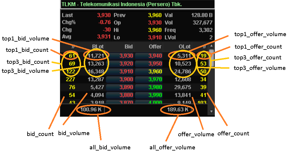

Bid offer variables illustration

top1_bid_volume — total volume on the bid at the best price, in shares
top1_bid_count — number of orders on the bid at the best price
top1_offer_volume — total volume on the offer at the best price, in shares
top1_offer_count — number of offer orders at the best price
top3_*, top5_*, top10_* — the same pattern across the 3, 5 and 10 best prices
all_bid_volume — total volume on the bid across all prices, in shares
all_bid_count — number of orders on the bid across all prices
all_offer_volume — total volume on the offer across all prices, in shares
all_offer_count — number of offer orders across all prices

Function forms are also available:

bid_volume(n)      : volume on the bid at the nth best price, where n: 1,2,3,...
bid_count(n)       : number of orders on the bid at the nth best price
offer_volume(n)    : volume on the offer at the nth best price
offer_count(n)     : number of orders on the offer at the nth best price

sum_bid_volume(n)   : total volume on the bid across the n best prices
sum_bid_count(n)    : number of orders on the bid across the n best prices
sum_offer_volume(n) : total volume on the offer across the n best prices
sum_offer_count(n)  : number of orders on the offer across the n best prices

Other variables

To check the value of a variable or test a formula, use the Formula Evaluator menu.

best_bid_price — the highest (best) bid price for the stock
best_offer_price — the lowest (best) offer price for the stock
blot — transaction volume executed at the bid price (ha-ki), in lots
slot — transaction volume executed at the offer price (ha-ka), in lots
bvol — transaction volume executed at the bid price, in shares
svol — transaction volume executed at the offer price, in shares
bfreq — transaction frequency at the bid price
sfreq — transaction frequency at the offer price
all_buy_volume / all_sell_volume — the same as bvol / svol
all_buy_freq / all_sell_freq — the same as bfreq / sfreq
broker_buyer_count — the number of brokers buying
broker_seller_count — the number of brokers selling
net_broker_buyer_count — the number of brokers with a net buy
net_broker_seller_count — the number of brokers with a net sell

Broker transaction variables

Available in the pattern top{1,3,5,10}_net_broker_{buyer,seller}_{volume,value,avg_price}:

top1_net_broker_buyer_volume     : net buy volume of the single largest broker, in shares
top1_net_broker_buyer_value      : net buy transaction value of the single largest broker
top1_net_broker_buyer_avg_price  : average net buy price of the single largest broker

The same pattern applies to top3_, top5_, top10_ and to the seller side, giving the full list:

top1_net_broker_buyer_volume    top1_net_broker_buyer_value    top1_net_broker_buyer_avg_price
top3_net_broker_buyer_volume    top3_net_broker_buyer_value    top3_net_broker_buyer_avg_price
top5_net_broker_buyer_volume    top5_net_broker_buyer_value    top5_net_broker_buyer_avg_price
top10_net_broker_buyer_volume   top10_net_broker_buyer_value   top10_net_broker_buyer_avg_price

top1_net_broker_seller_volume   top1_net_broker_seller_value   top1_net_broker_seller_avg_price
top3_net_broker_seller_volume   top3_net_broker_seller_value   top3_net_broker_seller_avg_price
top5_net_broker_seller_volume   top5_net_broker_seller_value   top5_net_broker_seller_avg_price
top10_net_broker_seller_volume  top10_net_broker_seller_value  top10_net_broker_seller_avg_price

Versions without the word net are available in the same pattern, covering _volume, _value and _avg_price:

top1_broker_buyer_volume    top1_broker_buyer_value    top1_broker_buyer_avg_price
top3_broker_buyer_volume    top3_broker_buyer_value    top3_broker_buyer_avg_price
top5_broker_buyer_volume    top5_broker_buyer_value    top5_broker_buyer_avg_price
top10_broker_buyer_volume   top10_broker_buyer_value   top10_broker_buyer_avg_price

top1_broker_seller_volume   top1_broker_seller_value   top1_broker_seller_avg_price
top3_broker_seller_volume   top3_broker_seller_value   top3_broker_seller_avg_price
top5_broker_seller_volume   top5_broker_seller_value   top5_broker_seller_avg_price
top10_broker_seller_volume  top10_broker_seller_value  top10_broker_seller_avg_price

Earlier-bar values for bid, offer and broker variables

The variables in the three sections above — bid_offer_variables, Other variables and Broker transaction variables — come from the live data feed rather than from a calculation over candle history.

For some past bars their value is not stored. When that happens, prev and prev_N return the current value instead of the value on the bar you asked for.

prev top5_net_broker_buyer_volume    ==> may return the same value as the
                                         current bar

So comparisons across bars on these variables are not yet dependable — the result can be a value compared against itself:

top5_net_broker_buyer_volume > prev top5_net_broker_buyer_volume
all_bid_volume > prev all_bid_volume

The same applies when these variables are used inside an sma, hhv, llv, sum or count subformula, since all of those read a value per bar.

Variables and functions computed from candle history, by contrast, support prev fully:

close > prev close
volume > prev volume
foreign > prev foreign
top_broker > prev_5 top_broker
rsi(14) < prev rsi(14)

To check whether a particular variable returns a different value on an earlier bar, use the Formula Evaluator menu.

We are preparing stored history for these variables, starting with the daily timeframe. This page will be updated once it is available.

Naming parts of a formula: `define` and `var`

A long formula is easier to read, and to change, when its parts have names. Write the named parts first, one per line, and finish with the criterion itself:

define body  close - open
define spike volume > 2 * sma(volume, 20)
spike and body > 0 and close > sma(close, 20)

This is exactly the same criterion as volume > 2 * sma(volume, 20) and close - open > 0 and close > sma(close, 20). Names work everywhere a formula does: in the Screener, Stock Scoring (end with a number instead of a criterion), Formula-Based Alerts, the Formula Evaluator and DataSahamBot charts.

There are two kinds of names.

`define`: a name for a formula

define name formula gives a formula a name. Wherever the name appears, the formula is worked out right there, on that bar, timeframe or stock. So a define can be used anywhere its formula could:

define body close - open

prev(body)                 ==> the previous bar's body
prev_3 body                ==> the body 3 bars ago
sma(body, 5)               ==> the average body over 5 bars
count(body > 0, 10)        ==> how many of the last 10 bars rose
body cross_up 0
weekly body                ==> this week's body: weekly close - weekly open
code:BBRI body             ==> BBRI's body

A define ends at the end of its line. To carry on to the next line, end the line with \; a line that ends inside an open bracket carries on by itself:

define band (hhv("high", 20) +
             llv("low", 20)) / 2
close > band

Several defines can share a line, separated by ;. A define can use the defines before it, a name can be defined only once, and a define never changes.

`var`: a value worked out once

var name = formula; works the formula out once, on the bar being screened, and keeps the result. Unlike a define, a var is one value, the same on every bar. A var can be given a new value later with = (:= works too). Each var line ends with ;:

var lim   = sma(close, 50);
var level = lim * 1.02;            ==> 2% above the MA 50
level = level + tick;              ==> and one tick more
close > level

`define` or `var`?

The difference shows whenever a name is read on other bars: by prev, val, a cross, or a function that works over several bars, such as sma, count, highest or prev_candle_index.

A define gives its formula on each of those bars.
A var gives the same single value on every one of them.

So a name that will be read on other bars must be a define. The screener refuses a var there, rather than return something that looks right and is not:

var m = close - open;
sma(m, 5) > 0
==> m is a var: sma() reads its formula on bar after bar, but a var is one value,
    the same on every bar. For a formula read bar by bar, write define m ... instead.

A var is fine as part of a formula that does change from bar to bar: count(close > lim, 10) counts the last 10 bars whose close was above today’s lim.

A rule of thumb: use define for anything that describes a bar (a body, a new high, a crossing), and var for a level worked out today (a target, a threshold, how many bars back something happened).

If you are used to TradingView, note that there every variable is a series; in TQL that is a define. For TradingView’s var (a value carried from bar to bar), see foreach below.

Names and built-in fields

A define or var may take the name of a built-in field, such as define close (high + low) / 2. From that line on, the name means yours. Only the name as you write it changes: built-in indicators such as rsi(14) still use the real close.

Giving a value to a name that was never declared is refused, which also catches a comparison written with a single =:

open = close
==> open is not declared: write var open = ... to make it. To compare, use == (close == open).

Comments

Text after // or # to the end of the line, and anything between /* and */, is ignored, including on the formula’s last line. It is a good place to say what each part is for.

Example: the Darvas box

This TradingView script draws a Darvas box. In Pine, every line is a series:

LL = lowest(low, boxp)
k1 = highest(high, boxp)
k2 = highest(high, boxp - 1)
k3 = highest(high, boxp - 2)
NH = valuewhen(high > k1[1], high, 0)
box1 = k3 < k2
TopBox = valuewhen(barssince(high > k1[1]) == boxp - 2 and box1, NH, 0)
BottomBox = valuewhen(barssince(high > k1[1]) == boxp - 2 and box1, LL, 0)

In TQL, with boxp = 5:

// Darvas box, boxp = 5
define newhigh high > prev highest(high, 5)        // a high above the 5 bars before
define formed  prev_candle_index(newhigh, 250) == 3 and highest(high, 3) < highest(high, 4) \
               and count(volume == 0, 4) == 0       // and the stock traded on those bars
var m         = prev_candle_index(formed, 250);  // bars since the box formed
var topbox    = val(high, m + 3);
var bottombox = val(lowest(low, 5), m);
// a breakout above the box
close > topbox

barssince(cond) is prev_candle_index(cond, 250): the bars since the condition last held, looking back up to 250 bars. (Pine looks back over the whole history.)
valuewhen(cond, src, 0) is val(src, prev_candle_index(cond, 250)).
newhigh and formed are read on earlier bars by prev_candle_index, so they are defines. m, topbox and bottombox are only needed for today, so they are vars.
When the box forms, the new high is always boxp - 2 bars before it, so the top of the box is simply the high m + 3 bars back.
On a DataSahamBot chart, /bike darvas draws the same box.
count(volume == 0, 4) == 0 is not in the Pine script. Days a stock was suspended have no bar in the data the screener reads, as on TradingView; the one bar without a trade is today’s, until the stock first trades. The check keeps a box from forming on that bar.

Carrying a value from bar to bar: `foreach`

Some indicators work out each bar from their own value on the bar before. Supertrend’s bands only move one way until a close breaks through them; a trailing stop only moves up. A define cannot do this, because it cannot use itself, and a var is a single value. foreach runs statements on every bar, the oldest first, and vars keep their values from one bar to the next:

var s = 0;
foreach last 10
{
    s = s + close;        // on each of the last 10 bars
}
s                         // the same as sum(close, 10)

foreach { ... } runs the statements inside on every bar of the stock’s history, from the oldest to the bar being screened. foreach last N { ... } runs them on the last N bars only.
On each bar, the formulas inside are read on that bar: close is that bar’s close, prev close the one before it, atr(10) the ATR as it was then.
Vars keep their values from one bar to the next. After the loop, a var holds its value at the bar being screened, and the formula after the loop uses it like any other var.
var a, b, c = 1; declares several vars at once. A var declared without a value has none yet: is_nan(x) is true until it is given one. That is how a loop knows it is on its first bar.
Only var lines and assignments go inside foreach, each ending with ;. Put defines before the loop. A loop cannot contain another loop.
foreach weekly { ... } runs on weekly bars; any timeframe can be named. A loop reads one timeframe, so a name with another timeframe inside it, such as weekly close in a daily loop, is refused.
A var is still one value, so prev x on a var is refused inside a loop too. To keep the previous bar’s value, copy it before changing it, as prev_dir = dir; does in the examples below.
return before the final formula is optional: return dir == 1 is the same as dir == 1.

A loop over the whole history takes longer the first time a formula runs; after that, the values up to the previous bar are kept, and only the latest bar is worked out again. foreach last 250 limits a loop to about a year of daily bars.

Loops also work in DataSahamBot charts, written on one line inside def(...).

Both examples below are also built in: supertrend() and chandelier_long() and the related functions. The loops show how they work, and are a starting point for variations of your own.

Example: Supertrend

Supertrend draws one line: below the price while the trend is up, above it while the trend is down. Its two bands are the bar’s midpoint plus and minus 3 ATR, and each is held in place: the upper band can move down but not up until a close breaks above it, and the lower band the other way round. When a close breaks the band in force, the trend turns.

// Supertrend(10, 3), as TradingView's built-in
var up, dn, prev_dir, dir = -1;   // dir: 1 = uptrend, -1 = downtrend
foreach
{
    var a   = atr(10);
    var mid = (high + low) / 2;
    var ub  = mid + 3 * a;        // the bands before they are held
    var lb  = mid - 3 * a;
    up = is_nan(up) or ub < up or prev close > up ? ub : up;   // moves down only, until a close above it
    dn = is_nan(dn) or lb > dn or prev close < dn ? lb : dn;   // moves up only, until a close below it
    prev_dir = dir;
    dir = dir == -1 and close > up ? 1 : dir == 1 and close < dn ? -1 : dir;
}
dir == 1 and prev_dir == -1       // turned up on this bar

Change the last line for other uses:

Last line	Gives
`dir == 1 and prev_dir == -1`	turned up on this bar (buy)
`dir == -1 and prev_dir == 1`	turned down on this bar (sell)
`dir == 1`	in an uptrend
`dir == 1 ? dn : up`	the Supertrend line itself, for Stock Scoring, the Formula Evaluator or a chart

Example: Chandelier Exit

Chandelier Exit hangs a long stop 3 ATR below the highest close of the last 22 bars, and a short stop 3 ATR above the lowest close. Each stop is held: the long stop only moves up while closes stay above it, and the short stop only moves down while closes stay below it. The trend turns up when a close crosses above the short stop, and down when a close crosses below the long stop.

// Chandelier Exit(22, 3), on closes
var long_stop, short_stop, prev_dir, dir = 1;
foreach
{
    var a  = 3 * atr(22);
    var ls = highest(close, 22) - a;                 // the stops before they are held
    var ss = lowest(close, 22) + a;
    var lp = is_nan(long_stop)  ? ls : long_stop;    // yesterday's stops
    var sp = is_nan(short_stop) ? ss : short_stop;
    long_stop  = prev close > lp ? max(ls, lp) : ls; // moves up only, while the close stays above it
    short_stop = prev close < sp ? min(ss, sp) : ss; // moves down only, while the close stays below it
    prev_dir = dir;
    dir = close > sp ? 1 : close < lp ? -1 : dir;
}
dir == 1 and prev_dir == -1       // turned up on this bar

This follows the widely used Chandelier Exit script on TradingView with its default of using closes for the highest and lowest. To use highs and lows instead, write highest(high, 22) and lowest(low, 22). The last line works the same way as in Supertrend; long_stop alone gives the stop level for a position you hold.

From Pine Script: `nz()` and the previous bar’s value

In Pine Script, a series that uses its own value on the previous bar is usually written with nz(), for example adding up price changes on the days volume falls and rises:

// Pine Script
ROC = roc(close, 1)
negVol = iff(volume < volume[1], nz(negVol[1], 0) + ROC, nz(negVol[1], 0))
posVol = iff(volume > volume[1], nz(posVol[1], 0) + ROC, nz(posVol[1], 0))

nz(negVol[1], 0) means “the value of negVol on the previous bar, or 0 if there is none yet”. In TQL this pattern is written with foreach: declare the var with a starting value of 0 before the loop, and inside the loop the var holds its value from the previous bar.

var neg_vol = 0;
var pos_vol = 0;
foreach
{
    var r = roc(1);
    neg_vol = volume < prev volume ? neg_vol + r : neg_vol;
    pos_vol = volume > prev volume ? pos_vol + r : pos_vol;
}
neg_vol > pos_vol

Pine Script	TQL
`nz(negVol[1], 0)`	`var neg_vol = 0;` before the loop, then `neg_vol` inside it
`iff(condition, a, b)`	`condition ? a : b`
`roc(close, 1)`	`roc(1)`
`volume[1]`, `close[1]`	`prev volume`, `prev close`

Change the last line to suit, for example neg_vol > 0. For Stock Scoring or the Formula Evaluator, end with just neg_vol to get its value.

Things to keep in mind:

The value is a running total from the first bar of the history. The number can differ from TradingView’s when the two platforms’ histories start on different dates, but its change from bar to bar is the same. To add up from a fixed point, write foreach last 250 (about a year of daily bars).
A var holds a single value, so ema(neg_vol, 255) cannot be written after the loop. If your Pine script uses an EMA signal line, work out the EMA inside the loop:

var neg_vol = 0;
var neg_ema;
foreach
{
    var r = roc(1);
    neg_vol = volume < prev volume ? neg_vol + r : neg_vol;
    neg_ema = is_nan(neg_ema) ? neg_vol : neg_ema + (neg_vol - neg_ema) * 2 / (255 + 1);
}
neg_vol > neg_ema

2 / (255 + 1) is the smoothing factor of a 255-period EMA. This EMA starts from the first value, as Pine’s ema definition does; a version seeded with an SMA differs only on the early bars.

Building your own formulas

Beyond the built-in functions, you can assemble calculations yourself. The key: sma, ema, aema, sum, hhv, llv and ranking accept a subformula that is a full expression, not merely a stock_attr name. Look at the definition of vwap above — it contains sum("volume * (high + low + close) / 3", N), a complete expression inside quotes.

This section shows how that works, using several widely known indicators.

Every indicator in this section is now available as its own function. For everyday use, call the function directly — it is shorter, faster, and less prone to typos. The long forms are kept here as worked examples, so you can apply the same pattern to indicators that do not yet have one.

Donchian Channel

The upper and lower Donchian bands are the highest and lowest values over the last N bars:

hhv("high", 20)                            ==> upper band
llv("low", 20)                             ==> lower band
(hhv("high", 20) + llv("low", 20)) / 2     ==> midline

Available directly as donchian_up(20), donchian_down(20) and donchian_mid(20).

VWMA — Volume Weighted Moving Average

A close-price average weighted by volume. The pattern matches the definition of vwap:

sum("volume * close", 20) / sum("volume", 20)

Available directly as vwma(20).

PPO and PVO

MACD expressed as a percentage, and the same measure applied to volume:

(ema("close", 12) - ema("close", 26)) / ema("close", 26) * 100
(ema("volume", 12) - ema("volume", 26)) / ema("volume", 26) * 100

Available directly as ppo(12, 26) and pvo(12, 26).

Awesome Oscillator

The difference between two simple moving averages of the median price. Since mid_price is already (high + low) / 2, this becomes:

sma("mid_price", 5) - sma("mid_price", 34)

Available directly as ao(5, 34).

Crossover and breakout signals

The signals people reach for — golden cross, death cross, breakout — are fundamentally a comparison between the previous bar and the current one. Writing them yourself lets you choose your own periods, and keeps the criterion readable.

The pattern is always the same: the condition did not hold on prev, and holds now — which is exactly what cross_up and cross_down check (see Crossing above).

Golden cross and death cross, MA 5–20

sma("close", 5) cross_up sma("close", 20)       ==> golden cross
sma("close", 5) cross_down sma("close", 20)     ==> death cross

Replace 5 and 20 with whatever periods suit your strategy, or swap sma for ema or aema.

MACD crossing the zero line

macd(12, 26) cross_up 0        ==> golden cross
macd(12, 26) cross_down 0      ==> death cross

MACD crossing its signal line — equivalent to the histogram changing sign

macd(12, 26) cross_up macd_signal(12, 26, 9)
macd_histogram(12, 26, 9) cross_down 0

Stochastic %K crossing %D

stoch_k(15, 3) cross_up stoch_d(15, 3, 3)
stoch_k(15, 3) cross_down stoch_d(15, 3, 3)

The same with the shorter names: stok(15, 3) xu stod(15, 3, 3).

Fractal breakout

high > up_fractal and prev close <= up_fractal      ==> breaking the upper fractal
low < down_fractal and prev close >= down_fractal   ==> breaking the lower fractal

Confirming across many moving averages at once

The ma_net_buy_sell_signal_count variable nets buy against sell signals across 12 moving averages, ranging from −12 to +12.

ma_net_buy_sell_signal_count >= 6     ==> most moving averages strengthening
ma_net_buy_sell_signal_count <= -6    ==> most weakening

Fibonacci retracement

There is no single fib() function in the app, and that is deliberate. A Fibonacci result depends entirely on which points are used as anchors: two people drawing lines on different swings get different numbers, and both are legitimate. So the anchors are yours to choose.

The arithmetic itself is simple. Once a peak and a trough are settled on:

peak   - (peak - trough) * ratio    ==> up swing, retracement measured down from the peak
trough + (peak - trough) * ratio    ==> down swing, retracement measured up from the trough

The ratios in common use are 0.236, 0.382, 0.5, 0.618 and 0.786. The 0.5 is not a Fibonacci ratio at all, merely the midpoint, but it has long since become conventional.

Anchored on swing pivots

The closest thing to the line you would draw yourself on a chart:

pivot_low_bars(5) > pivot_high_bars(5)
  ? pivot_high(5) - (pivot_high(5) - pivot_low(5)) * 0.618
  : pivot_low(5) + (pivot_high(5) - pivot_low(5)) * 0.618

The ? : operator settles the direction of the swing. If the trough is older than the peak, price has just climbed, so the retracement is measured down from the peak.

Anchored on an N-bar range

Simpler, using the highest and lowest price over the last N bars:

llvbars("low", 60) > hhvbars("high", 60)
  ? hhv("high", 60) - (hhv("high", 60) - llv("low", 60)) * 0.618
  : llv("low", 60) + (hhv("high", 60) - llv("low", 60)) * 0.618

Screening for a stock that touched a level

low <= pivot_high(5) - (pivot_high(5) - pivot_low(5)) * 0.618
and close > pivot_high(5) - (pivot_high(5) - pivot_low(5)) * 0.618

==> price dipped through the 61.8% level during the day, then closed back above it.

A shortcut: how far price has already retraced

For screening, what is usually wanted is not the level itself but how far price has retraced within its swing. That number is already available through stoch_k with a smoothing period of 1:

stoch_k(60, 1)     ==> where price sits within the 60-bar range, as a percentage

On an up swing, a retracement of R means stoch_k reads 100 − R:

Retracement	`stoch_k(N, 1)`
23.6%	76.4
38.2%	61.8
50.0%	50.0
61.8%	38.2
78.6%	21.4

So “retraced close to 61.8% of the 60-bar swing” is simply:

stoch_k(60, 1) > 35 and stoch_k(60, 1) < 42

Patterns with no function

Some calculations have no function name but are still easy to write with the same pattern.

Distance from a moving average — useful for screening out stocks that have run too far from their average.

(close - sma("close", 20)) / sma("close", 20) * 100 > 5

Volume spike

volume > sma("volume", 20) * 2

The average of an expression — anything you can write as a single-bar expression, you can average.

sma("(high - low)", 14)                  ==> average daily range
sma("(close - open) / open * 100", 5)    ==> average intrabar change
sum("top_broker_hist * close", 5)        ==> 5-day broker accumulation value

Ratios across timeframes

volume / weekly volume                   ==> daily volume as a share of weekly
close / weekly sma("close", 4)           ==> price against the 4-week average

Screener formula examples

Higher high higher low

prev high < high and prev low < low

Inside bar

prev high > high and prev low < low

Golden cross MA 5-20 (the MA 5 line crossing above MA 20)

prev sma(5) < prev sma(20) and sma(5) > sma(20)

MACD rising

prev macd < macd and macd > 0

Three white soldiers

prev_2 close > prev_2 open
and prev close > prev open
and close > open

The 10 highest accumulation stocks by top-5-net-broker-accumulation value

ranking("top_broker_hist * daily_price_avg") <= 10

Stochastic %K crossing %D from below

prev stoch_k < prev stoch_d and stoch_k > stoch_d

Stocks that have just set a 25-day high

aroon_up(25) == 100

A strong uptrend by Aroon — the high is recent, the low is old

aroon_up(25) > 70 and aroon_down(25) < 30

Aroon Oscillator crossing up — a turn from down to up

prev aroon_osc(25) < 0 and aroon_osc(25) > 0

A new trend forming, not yet overbought

aroon_up(14) > 70 and aroon_down(14) < 30 and rsi < 70

Accumulation by Chaikin Oscillator, with above-average volume

chaikin_osc(3, 10) > 0
and prev chaikin_osc(3, 10) < 0
and volume > sma("volume", 20)

Accumulation divergence — price sets a new high while accumulation falls away

close == hhv("close", 20) and adl < prev_5 adl

Double confirmation — Chaikin positive alongside top 5 broker accumulation

chaikin_osc(3, 10) > 0 and top_broker_hist > 0

Restricting results to members of a particular index

code_index("ISSI") and close > sma("close", 20)

Liquid stocks with large transaction value — 5-day average above 1 billion

sma("value", 5) > 1B

A combination: price above the weekly SMA26, MACD histogram rising below the centre line, and Stochastic %K below 19 crossing %D from below.

close > weekly sma("close", 26)
and macd_histogram < 0
and prev_2 macd_histogram < prev macd_histogram
and prev macd_histogram < macd_histogram
and stoch_k < 19
and prev stoch_k < prev stoch_d
and stoch_k > stoch_d

Complete screener examples

The section above shows single conditions. This one assembles them into whole screeners, together with the tradeability filter that is most often left out.

One thing to be clear about first: a screener filters, it does not predict. It narrows hundreds of stocks down to the few meeting conditions you set yourself. When to enter, when to leave, and where to stop remain your decisions — and that is where the result is actually determined. The formulas below are examples to study and test, not recommendations.

The round-trip cost that is easy to forget

Every trade carries two costs before the price moves at all: crossing one price fraction, and the broker fee together with the sales tax. The exchange’s price fraction is tiered, so its weight relative to price differs sharply between levels:

Price	Fraction	1 fraction	+ fees ±0.4%	Share of a 2% target
Rp 100	1	1.00%	1.40%	70%
Rp 200	2	1.00%	1.40%	70%
Rp 500	5	1.00%	1.40%	70%
Rp 1,200	5	0.42%	0.82%	41%
Rp 1,999	5	0.25%	0.65%	33%
Rp 4,999	10	0.20%	0.60%	30%
Rp 10,000	25	0.25%	0.65%	33%

The cost is heaviest just above each fraction boundary: at Rp 200, Rp 500, Rp 2,000 and Rp 5,000 a single fraction is a full 1% or 0.5% of the price. On a 2% target that consumes 30% to 70% of the target before the stock does anything.

The consequence is clearest when you work out how often a strategy must be right merely to break even:

Target	Stop	Must be right
2%	2%	72.5%
2%	1%	63.3%
3%	1.5%	53.3%
7%	3%	39.0%
10%	5%	37.7%

This is why a 5–10% target over a few days is generally easier to live with than 2–3% within a day. Not because it is easier to predict, but because the fixed cost weighs proportionally far less.

The tradeability filter

All the examples below open with the same line. It discards stocks that trade too thinly, and stocks whose price fraction is too expensive relative to their price:

value > 5B and tick / close * 100 < 0.30

The tick variable holds the price fraction in force, so tick / close * 100 gives the cost of one fraction as a percentage directly. No need to guess at a price floor.

Intraday momentum

Finding stocks moving on volume above their own habit, but not yet run too far:

value > 5B
and tick / close * 100 < 0.30
and projected_volume > sma("volume", 20) * 2
and change_percent > 1
and change_percent < 6
and bvol > svol

projected_volume is the key piece: it estimates volume through to the end of the session from the pace so far, so “unusual volume” can be detected at ten in the morning rather than only near the close. The change_percent < 6 ceiling discards stocks whose move is already spent. bvol > svol says more business is being done on the demand side.

Breakout with confirmation

For a two- to three-day hold:

value > 5B
and tick / close * 100 < 0.30
and close > prev hhv("high", 20)
and volume > sma("volume", 20) * 2
and slope(50) > 0
and linreg_r2(50) > 0.5
and close > sma("close", 200)

linreg_r2 is what separates a breakout from an orderly base from a breakout out of pure chop. Without that line the two look identical.

A pullback inside an orderly trend

Buying weakness within strength, while waiting for the turn:

value > 5B
and tick / close * 100 < 0.30
and slope(60) > 0
and linreg_r2(60) > 0.6
and close > sma("close", 200)
and rsi < 40
and close > prev close

That last line waits for price to turn back up rather than catching a falling knife.

Scalping: 5-minute momentum

For trades opened and closed within the day, watched on 5-minute bars:

value > 5B
and tick / close * 100 < 0.30
and 5min close > 5min ema(20)
and 5min rsi(14) > 55
and 5min volume > 5min sma("volume", 20) * 2

The 5min prefix reads 5-minute bars, while value remains today’s transaction value for the whole day. Price above the 20-bar EMA with RSI above 55 marks upward momentum on the minute scale; the last line asks for the current 5-minute bar’s volume to be at least twice its average. Drop that line if too few stocks come through, especially early in the session when the 5-minute bar has only just started.

For scalping, keep the round-trip cost above in mind: small targets make the tradeability filter matter all the more.

Swing: Supertrend changing direction

A buy signal when Supertrend turns up on this bar:

value > 5B
and tick / close * 100 < 0.30
and supertrend_dir(10, 3) cross_up 0

A sell signal, the reverse, when Supertrend turns down:

value > 5B
and tick / close * 100 < 0.30
and supertrend_dir(10, 3) cross_down 0

supertrend_dir is 1 while the trend is up and -1 while it is down, so crossing 0 is the moment the direction changes. How Supertrend works is explained in the Supertrend example above. To hold positions longer and change direction less often, raise the factor, for example supertrend_dir(10, 4). The line itself can be seen on DataSahamBot charts, for example /chart bbca d supertrend.

Swing: an uptrend with RSI crossing 50

Waiting for momentum to recover inside an uptrend that is already in place:

value > 5B
and tick / close * 100 < 0.30
and close > sma(20)
and sma(20) > sma(50)
and rsi(14) cross_up 50

Price above the 20-day SMA and the 20-day SMA above the 50-day establish the uptrend; rsi(14) cross_up 50 is the moment momentum strengthens again after a dip, an earlier entry than waiting for a breakout.

Each example above can be saved as a Formula-Based Alert, so you are notified when a stock newly meets its criteria, whether a buy or a sell signal.

Making them your own

Every number above — 20, 50, 60, 5B, 0.30, 40 — is a choice, not a fixture. Change them and test against the stocks you actually follow. A good screener reflects how you read the market, not how someone else does.

For minute-by-minute watching there is also a far shorter form, such as finding stocks with at least one billion rupiah of haka in the last minute:

1min slot * 100 * close >= 1B

Questions that come up often

These are the things most frequently asked, with their answers.

The formula looks right but the result is always empty

The most common cause: hhv, highest, llv and lowest already include the current bar. So this is almost never true:

close > hhv("close", 20)        ==> almost always false

If today really is the highest close in 20 bars, then hhv("close", 20) equals close, which makes close > hhv(...) false. Compare against the earlier bars instead:

close > prev hhv("close", 19)   ==> breaking above the previous 19 bars' high

To say “today is the highest of the last 20 bars” there is a shorter form:

hhvbars("close", 20) == 0

The multiplication sign

Multiplication is written with an asterisk *, not the letter x:

volume >= 2 * ema("volume", 5)     ==> correct
volume >= 2 x ema("volume", 5)     ==> not valid

The `tick` variable at fraction boundaries

tick holds the price fraction in force at the current price. Because the fraction changes at Rp 200, Rp 500, Rp 2,000 and Rp 5,000, a calculation that crosses one of those boundaries can give an unexpected result.

Take a stock that opens at 1,980 and closes at 2,020:

close >= open + 5 * tick
2020 >= 1980 + 5 * 10       ==> 2020 >= 2030, which is false

The rise actually spans two fraction tiers, but tick at the close is 10. For a range that may cross a boundary, a percentage is safer:

close >= open * 1.02

The bandarmology figure differs when you add it up yourself

The 20 days top 5 broker accumulation shown on the Bandarmology tab is calculated like this:

sum("top_broker_hist * avg_price", 20)

Reading it through:

top_broker_hist — the net buy volume of the top 5 brokers minus their net sell volume, in shares
avg_price — the average transaction price on that bar, so the product is a transaction value
the two are summed over the last 20 bars

Summing top_broker_hist on its own, without multiplying by price, gives a different number — its unit is shares, not rupiah.

When broker transaction data is updated

top_broker_hist and the other broker transaction variables are updated after the market closes, at around 18:00 on each trading day, and reach back roughly six months.

What the screener scans

Stocks, warrants and ETFs are all scanned when they meet the criteria. Indices, sectoral indices, world indices, commodities and currencies are not included in screener results.

How often results refresh

During trading hours the screener refreshes its results automatically every minute.

Why formulas should be light and fast

Each screener and alert runs one at a time for the same ID. While a check is still running, the next scheduled check of that screener or alert is skipped rather than run alongside it. So a slow formula is checked less often than its schedule says: an alert with a 15-second interval that takes 40 seconds per run only runs about once a minute, and a condition that holds only briefly can be missed.

To keep formulas light:

Use a built-in function when one exists. supertrend(10, 3) is far faster than a foreach loop that produces the same value.
Limit the data range. Write foreach last 250 rather than looping over the whole history, and keep the periods of sum("...", n), count("...", n) and other functions that work out a sub-formula on every bar to what you need.
Use ranking() only when you need it. It works out its formula for every stock on the exchange, not just the one being checked.
Include a cheap filter, such as value > 5B. Stocks that fail it don’t need the heavy part of the formula worked out.
Name heavy parts you use more than once with define, so they are not worked out again in each place.
Choose an alert interval that fits. A formula based on daily bars does not need checking every second; a 1-minute interval is enough.

An easy test: run the formula in the Screener first. If results take several seconds to appear, an alert with the same formula will run slowly too.

If you are still stuck

Send a description of the condition you are looking for to idx.datasaham@gmail.com. Describe what you want to find rather than the formula, and we will help you write it.

Boolean Expression

Expression hierarchy

Number notation

Conditional operator

Stock Expression

candle_selector

A whole formula on an earlier bar: prev()

timeframe

target

Writing parameters

stock_attr list

Short forms with a standard period

Shorthand names

stock_attr definitions

stock_function list

stock_function definitions

Maths functions

Swing pivots

Trade book functions

Accurate period limits

Boolean functions

Crossing: cross_up and cross_down

stock_fundamental_attr

bid_offer_variables

Other variables

Broker transaction variables

Earlier-bar values for bid, offer and broker variables

Naming parts of a formula: define and var

define: a name for a formula

var: a value worked out once

define or var?

Names and built-in fields

Comments

Example: the Darvas box

Carrying a value from bar to bar: foreach

Example: Supertrend

Example: Chandelier Exit

From Pine Script: nz() and the previous bar’s value

Building your own formulas

Donchian Channel

VWMA — Volume Weighted Moving Average

PPO and PVO

Awesome Oscillator

Crossover and breakout signals

Fibonacci retracement

Patterns with no function

Screener formula examples

Complete screener examples

The round-trip cost that is easy to forget

The tradeability filter

Intraday momentum

Breakout with confirmation

A pullback inside an orderly trend

Scalping: 5-minute momentum

Swing: Supertrend changing direction

Swing: an uptrend with RSI crossing 50

Making them your own

Questions that come up often

The formula looks right but the result is always empty

The multiplication sign

The tick variable at fraction boundaries

The bandarmology figure differs when you add it up yourself

When broker transaction data is updated

What the screener scans

How often results refresh

Why formulas should be light and fast

If you are still stuck

Ready to start analysing today?

A whole formula on an earlier bar: `prev()`

Crossing: `cross_up` and `cross_down`

Naming parts of a formula: `define` and `var`

`define`: a name for a formula

`var`: a value worked out once

`define` or `var`?

Carrying a value from bar to bar: `foreach`

From Pine Script: `nz()` and the previous bar’s value

The `tick` variable at fraction boundaries